How To Change Chart Labels In Excel

Alter centrality labels in a chart

Excel for Microsoft 365 Word for Microsoft 365 Outlook for Microsoft 365 PowerPoint for Microsoft 365 Excel 2021 Word 2021 Outlook 2021 PowerPoint 2021 Excel 2019 Word 2019 Outlook 2019 PowerPoint 2019 Excel 2016 Give-and-take 2016 Outlook 2016 PowerPoint 2016 Excel 2013 Word 2013 Outlook 2013 PowerPoint 2013 More than...Less

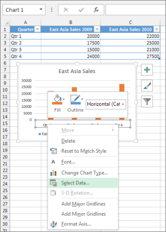
In a chart yous create, axis labels are shown below the horizontal (category, or "Ten") axis, adjacent to the vertical (value, or "Y") axis, and adjacent to the depth axis (in a 3-D nautical chart). Your chart uses text from its source information for these centrality labels.

Don't misfile the horizontal centrality labels—Qtr 1, Qtr two, Qtr 3, and Qtr iv, as shown below, with the legend labels beneath them—Eastern asia Sales 2009 and Eastern asia Sales 2010.

Change the text of the labels

1. Click each jail cell in the worksheet that contains the label text you lot want to change.

2. Type the text y'all want in each cell, and press Enter.

   

   As you change the text in the cells, the labels in the chart are updated.

To go on the text in the source data on the worksheet the way it is, and just create custom labels, you can enter new characterization text that'south independent of the worksheet information:

1. Right-click the category labels yous want to change, and click Select Data.

1. In the Horizontal (Category) Axis Labels box, click Edit.

2. In the Axis label range box, enter the labels yous want to use, separated past commas.

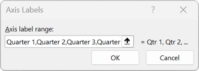
For example, type Quarter ane ,Quarter 2,Quarter 3,Quarter iv.

Alter the format of text and numbers in labels

To modify the format of text in category axis labels:

1. Right-click the category axis labels you want to format, and click Font.

2. On the Font tab, cull the formatting options yous want.

3. On the Character Spacing tab, choose the spacing options you want.

To change the format of numbers on the value axis:

1. Right-click the value axis labels you want to format.

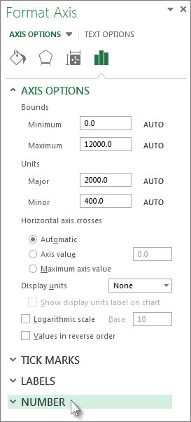
2. Click Format Axis.

3. In the Format Axis pane, click Number.

   Tip:If you don't meet the Number department in the pane, brand certain you've selected a value centrality (information technology'due south normally the vertical axis on the left).

   

4. Choose the number format options you want.

   

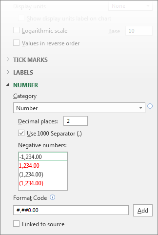
   If the number format you choose uses decimal places, you can specify them in the Decimal places box.

5. To continue numbers linked to the worksheet cells, check the Linked to source box.

   Note:Before y'all format numbers as percentages, make certain that the numbers shown on the chart have been calculated every bit percentages in the worksheet, or are shown in decimal format like 0.i. To calculate percentages on the worksheet, split up the amount past the total. For case, if you enter =ten/100 and format the outcome 0.1 equally a per centum, the number is correctly shown as x%.

Tip:An axis label is different from an axis title, which you can add together to describe what'south shown on the axis. Axis titles are not automatically shown in a nautical chart. To add them, see Add or remove titles in a nautical chart.

Need more assistance?

Source: https://support.microsoft.com/en-us/topic/change-axis-labels-in-a-chart-1c32436b-fb12-450b-aefa-cc7e4584456a

Posted by: espinozaexuld1949.blogspot.com

Share this post